


Analyzing eye-movement data
About this tutorial
We're going to analyze pupil-size data from an auditory-working-memory experiment. This data is taken from Mathôt (2018), and you can find the data and experimental materials here.
In this experiment, the participant first hears a series of digits; we will refer to this period as the sounds trace. The number of digits (set size) varies: 3, 5, or 7. Next, there is a retention interval during which the participant keeps the digits in memory; we will refer to this period as the retention trace. Finally, the participant enters the response.
We will analyze pupil size during the sounds and retention traces as a function of set size. As reported by Kahneman and Beatty (1966), and as we will also see during this tutorial, the size of the pupil increases with set size.
This tutorial makes use of the eyelinkparser module, which can be installed with pip:
pip install python-eyelinkparser
The data has been collected with an EyeLink 1000 eye tracker.
Designing an experiment for easy analysis
EyeLink data files (and data files for most other eye trackers) correspond to an event log; that is, each line corresponds to some event. These events can be gaze samples, saccade onsets, user messages, etc.
For example, a start_trial user message followed by four gaze samples might look like this:
MSG 451224 start_trial
451224    517.6   388.9  1691.0 ...
451225    517.5   389.1  1690.0 ...
451226    517.3   388.9  1692.0 ...
451227    517.1   388.7  1693.0 ...
When designing your experiment, it's important to send user messages in such a way that your analysis software, in this case eyelinkparser, knows how to interpret them. If you do, then data analysis will be easy, because you will not have to write a custom script to parse the data file from the ground up.
If you use OpenSesame/ PyGaze, most of these messages, with the exception of phase messages, will by default be sent in the below format automatically.
Trials
The following messages indicate the start and end of a trial. The trialid argument is optional.
start_trial [trialid]
end_trial
Variables
The following message indicates a variable and a value. For example, var response_time 645 would tell eyelinkparser that the variable response_time has the value 645 on that particular trial.
var [name] [value]
Phases
Phases are named periods of continuous data. Defining phases during the experiment is the easiest way to segment your data into different epochs for analysis.
The following messages indicate the start and end of a phase. A phase is automatically ended when a new phase is started.
start_phase [name]
end_phase [name]
For each phase, four columns of type SeriesColumn will be created with information about fixations:
fixxlist_[phase name]is a series of X coordinatesfixylist_[phase name]is a series of Y coordinatesfixstlist_[phase name]is a series of fixation start timesfixetlist_[phase name]is a series of fixation end timesblinkstlist_[phase name]is a series of blink start timesblinketlist_[phase name]is a series of blink end times
Additionally, four columns will be created with information about individual gaze samples:
xtrace_[phase name]is a series of X coordinatesytrace_[phase name]is a series of Y coordinatesttrace_[phase name]is a series of time stampsptrace_[phase name]is a series of pupil sizes
Analyzing data
Parsing
We first define a function to parse the EyeLink data; that is, we read the data files, which are in .asc text format, into a DataMatrix object.
We define a get_data() function that is decorated with @fnc.memoize() such that parsing is not redone unnecessarily (see memoization).
from datamatrix import (
  operations as ops,
  functional as fnc,
  series as srs
)
from eyelinkparser import parse, defaulttraceprocessor


@fnc.memoize(persistent=True)
def get_data():

    # The heavy lifting is done by eyelinkparser.parse()
    dm = parse(
        folder='data',           # Folder with .asc files
        traceprocessor=defaulttraceprocessor(
          blinkreconstruct=True, # Interpolate pupil size during blinks
          downsample=10,         # Reduce sampling rate to 100 Hz,
          mode='advanced'        # Use the new 'advanced' algorithm
        )
    )
    # To save memory, we keep only a subset of relevant columns.
    dm = dm[dm.set_size, dm.correct, dm.ptrace_sounds, dm.ptrace_retention,
            dm.fixxlist_retention, dm.fixylist_retention]
    return dm
We now call this function to get the data as a a DataMatrix. If you want to clear the cache, you can call get_data.clear() first.
Let's also print out the DataMatrix to get some idea of what our data structure looks like. As you can see, traces are stored as series, which is convenient for further analysis.
dm = get_data()
print(dm)
Output:
........../home/sebastiaan/anaconda3/envs/pydata/lib/python3.10/site-packages/datamatrix/series.py:1837: RuntimeWarning: Mean of empty
slice
return fnc(a.reshape(-1, by), axis=1)
[32m⠏[0m Generating....................................................................+----+---------+-----------------------+-----------------------+----------------------------+----------------------------+----------+
| # | correct | fixxlist_retention | fixylist_retention | ptrace_retention | ptrace_sounds | set_size |
+----+---------+-----------------------+-----------------------+----------------------------+----------------------------+----------+
| 0 | 1 | [525.9 529.7 ... nan] | [382.9 379.8 ... nan] | [1810. 1810.3 ... 1908.2] | [1655.6 1657.1 ... nan] | 5 |
| 1 | 1 | [528.9 527.7 ... nan] | [386.4 385.8 ... nan] | [1644.6 1648.7 ... 1673.4] | [1717.3 1718.5 ... nan] | 3 |
| 2 | 1 | [521.4 523. ... nan] | [377.3 367.9 ... nan] | [1787. 1791.4 ... 1719.3] | [1471.8 1470.4 ... 1785.3] | 7 |
| 3 | 1 | [523.2 513.9 ... nan] | [382.6 379.7 ... nan] | [1773.5 1774.8 ... 1752.5] | [1857.7 1859.1 ... nan] | 3 |
| 4 | 1 | [522.1 531.6 ... nan] | [373.5 376.1 ... nan] | [1939.2 1939.6 ... 1802.7] | [1847.2 1849.6 ... 1938.7] | 7 |
| 5 | 1 | [521. 526.9 ... nan] | [379.1 384.2 ... nan] | [1867.4 1867.9 ... 1768.4] | [1615.9 1619.3 ... 1870.6] | 7 |
| 6 | 1 | [520.8 532.5 ... nan] | [387.5 377.8 ... nan] | [1675.2 1674.1 ... 1581.4] | [1826.5 1821.8 ... nan] | 5 |
| 7 | 1 | [527.5 527. ... nan] | [396. 390.3 ... nan] | [1766.5 1766.7 ... 1682.2] | [1728.6 1726.7 ... nan] | 3 |
| 8 | 1 | [518.4 526.1 ... nan] | [391.8 388.3 ... nan] | [1733.3 1736.7 ... 1730.2] | [1636. 1637.6 ... 1729.3] | 7 |
| 9 | 0 | [528.2 541.3 ... nan] | [382.7 386.9 ... nan] | [1692. 1692.8 ... nan] | [1533. 1534.5 ... 1693.6] | 7 |
| 10 | 1 | [528.4 525.9 ... nan] | [388.3 378.2 ... nan] | [1602.2 1601.3 ... 1575.9] | [1789.2 1793.1 ... 1602.1] | 7 |
| 11 | 0 | [525. 519.7 ... nan] | [386.7 383.8 ... nan] | [1742.5 1740.1 ... 1559.5] | [1696.8 1700.6 ... 1746.8] | 7 |
| 12 | 1 | [503.1 514.6 ... nan] | [376.2 377.3 ... nan] | [1668.9 1668.8 ... nan] | [1667.6 1667.6 ... nan] | 5 |
| 13 | 1 | [517.2 511.3 ... nan] | [387.1 386. ... nan] | [1609.5 1602.3 ... 1584.3] | [1479.8 1477.9 ... 1609.2] | 7 |
| 14 | 1 | [507.6 502.5 ... nan] | [388.4 386.2 ... nan] | [1475.4 1473.7 ... 1490.7] | [1481.9 1477.6 ... nan] | 3 |
| 15 | 1 | [508.6 507.9 ... nan] | [387. 382.8 ... nan] | [1494.8 1494.2 ... 1522.1] | [1522.4 1518.7 ... 1495.4] | 7 |
| 16 | 1 | [498.6 509.6 ... nan] | [386.1 389.7 ... nan] | [1550.4 1550.3 ... 1385.9] | [1651.6 1649.1 ... nan] | 3 |
| 17 | 1 | [510.2 500.9 ... nan] | [387. 380.8 ... nan] | [1557.6 1559. ... 1532.] | [1537.8 1534. ... nan] | 3 |
| 18 | 1 | [521.7 512.4 ... nan] | [382.8 382.5 ... nan] | [1523.1 1521.9 ... 1409.6] | [1471.8 1472.6 ... nan] | 5 |
| 19 | 1 | [517.4 515.4 ... nan] | [386.5 380.5 ... nan] | [1500.1 1502. ... 1498.4] | [1530.4 1531. ... nan] | 5 |
+----+---------+-----------------------+-----------------------+----------------------------+----------------------------+----------+
(+ 55 rows not shown)
Preprocessing
Next, we do some preprocessing of the pupil-size data.
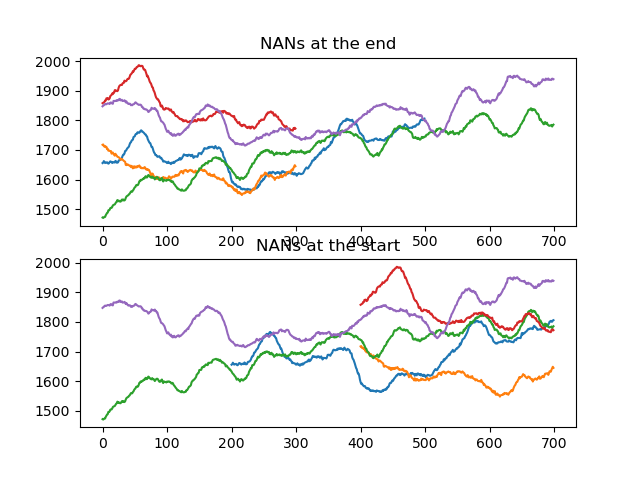
We are interested in two traces, sounds and retention. The length of sounds varies, depending on how many digits were played back. The shorter traces are padded with nan values at the end. We therefore apply srs.endlock() to move the nan padding to the beginning of the trace.
To get some idea of what this means, let's plot pupil size during the sounds trace for the first 5 trials, both with and without applying srs.endlock().
from matplotlib import pyplot as plt
from datamatrix import series as srs

plt.figure()
plt.subplot(211)
plt.title('NANs at the end')
for pupil in dm.ptrace_sounds[:5]:
    plt.plot(pupil)
plt.subplot(212)
plt.title('NANs at the start')
for pupil in srs.endlock(dm.ptrace_sounds[:5]):
    plt.plot(pupil)
plt.show()
Next, we concatenate the (end-locked) sounds and retention traces, and save the result as a series called pupil.
dm.pupil = srs.concatenate(
    srs.endlock(dm.ptrace_sounds),
    dm.ptrace_retention
)
We then perform baseline correction. As a baseline, we use the first two samples of the sounds trace. (This trace still has the nan padding at the end.)
dm.pupil = srs.baseline(
    series=dm.pupil,
    baseline=dm.ptrace_sounds,
    bl_start=0,
    bl_end=2
)
And we explicitly set the depth of the pupil trace to 1200, which given our original 1000 Hz signal, downsampled 10 ×, corresponds to 12 s.
dm.pupil.depth = 1200
Analyzing pupil size
And now we plot the pupil traces for each of the three set sizes!
import numpy as np


def plot_series(x, s, color, label):

    se = s.std / np.sqrt(len(s))
    plt.fill_between(x, s.mean-se, s.mean+se, color=color, alpha=.25)
    plt.plot(x, s.mean, color=color, label=label)


x = np.linspace(-7, 5, 1200)
dm3, dm5, dm7 = ops.split(dm.set_size, 3, 5, 7)

plt.figure()
plt.xlim(-7, 5)
plt.ylim(-150, 150)
plt.axvline(0, linestyle=':', color='black')
plt.axhline(1, linestyle=':', color='black')
plot_series(x, dm3.pupil, color='green', label='3 (N=%d)' % len(dm3))
plot_series(x, dm5.pupil, color='blue', label='5 (N=%d)' % len(dm5))
plot_series(x, dm7.pupil, color='red', label='7 (N=%d)' % len(dm7))
plt.ylabel('Pupil size (norm)')
plt.xlabel('Time relative to onset retention interval (s)')
plt.legend(frameon=False, title='Memory load')
plt.show()
Output:
/home/sebastiaan/anaconda3/envs/pydata/lib/python3.10/site-packages/numpy/lib/nanfunctions.py:1879: RuntimeWarning: Degrees of
freedom <= 0 for slice.
var = nanvar(a, axis=axis, dtype=dtype, out=out, ddof=ddof,
[32m⠦[0m Generating.../home/sebastiaan/anaconda3/envs/pydata/lib/python3.10/site-packages/datamatrix/_datamatrix/_seriescolumn.py:130:
RuntimeWarning: Mean of empty slice
return nanmean(self._seq, axis=0)
[32m⠦[0m Generating...
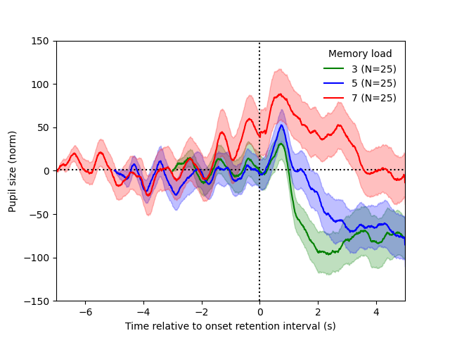
And a beautiful replication of Kahneman & Beatty (1966)!
Analyzing fixations
Now let's look at fixations during the retention phase. To get an idea of how the data is structured, we print out the x, y coordinates of all fixations of the first two trials.
for i, row in zip(range(2), dm):
    print('Trial %d' % i)
    for x, y in zip(
        row.fixxlist_retention,
        row.fixylist_retention
    ):
        print('\t', x, y)
Output:
Trial 0
     525.9 382.9
     529.7 379.8
     531.2 378.7
     526.2 381.9
     529.1 388.7
     nan nan
     nan nan
     nan nan
     nan nan
     nan nan
     nan nan
     nan nan
     nan nan
Trial 1
     528.9 386.4
     527.7 385.8
     530.8 383.9
     528.7 381.6
     530.0 379.0
     nan nan
     nan nan
     nan nan
     nan nan
     nan nan
     nan nan
     nan nan
     nan nan
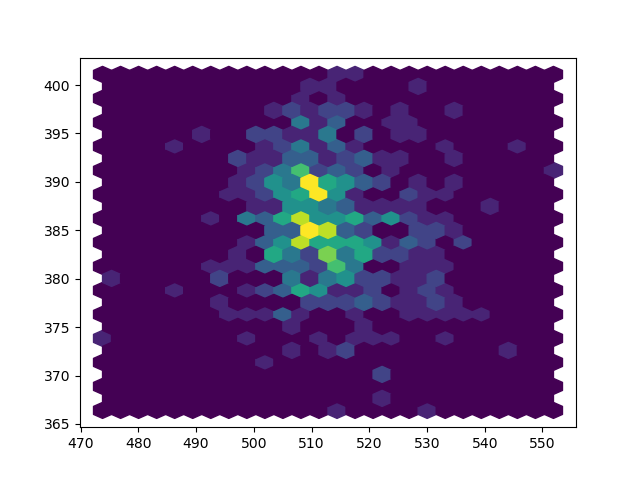
A common way to plot fixation distributions is as a heatmap. To do this, we need to create numpy arrays from the fixxlist_retention and fixylist_retention columns. This will result in two 2D arrays, whereas plt.hexbin() expects two 1D arrays. So we additionally flatten the arrays.
The resulting heatmap clearly shows that fixations are clustered around the display center (512, 384), just as you would expect from an experiment in which the participant needs to maintain central fixation.
import numpy as np

x = np.array(dm.fixxlist_retention)
y = np.array(dm.fixylist_retention)
x = x.flatten()
y = y.flatten()
plt.hexbin(x, y, gridsize=25)
plt.show()
References
- Kahneman, D., & Beatty, J. (1966). Pupil diameter and load on memory. Science, 154(3756), 1583–1585. https://doi.org/10.1126/science.154.3756.1583
- Mathôt, S., (2018). Pupillometry: Psychology, Physiology, and Function. Journal of Cognition. 1(1), p.16. https://doi.org/10.5334/joc.18